For sound generation in music synthesizers and industrial systems, often a precise sine wave is required. There are several methods to do this like the table based approximation used with classical DDS: The sine wave is stored in a RAM/ROM and directly read with an address counter derived from an accumulator representing the phase. These tables can easily be generated by e.g. an Excel sheet or also with MATLAB. Often only 90 degrees of the sine wave are stored and the values for other angles are derived by angle mapping and eventual level inversion. Here we can find two possibilities to store the values:

Representation of the phase vector in DDS

Most people use the borders of the focused region when defining the phase such as 0.0, 1.0, 2.0, 3.0, ... (n/4)-1 und repeat the curve backwards starting from the point n/4. This leads to 32 points in this case with the coordinates [0,1,2,3,4,5,6,7] and [8,7,6,5,4,3,2,1] which are repeated aging with inverted sign for angles beyond 180 degrees. This means the fundamental element starts at the angles 0, 90, 180 and 270 and does not include the last point of the area not to get this point twice. So the phases are p = 0, 1/n, 2/n ... (n-1)/n. It is important to mention that the division required to find the relative angle has to be performed with "n" and not with "n-1", what some people do. The dots generated this way, first cover a full period with 17 values / 9 values  0…180° = π. There are two slightly different quarters which are not symmetrical to each other. Another bit is required to represent the phase vector because of the (0…7) / (1…8) issue.

From the point of the ease of calculation and symmetry purposes it seems more appropriate to focus the mid of the ranges defined by the digital virtual phase 0 ... n-1. This leads in (this case) to 8 points in each quarter which are totally identical. The digital value 0 addressing the first dot represents it's region by the average value of the region and the value 7 does the same for the region between point 7 and point 8. To get the right value, a correction of Phase/n has to added to the phase vector. Thus the phase values are p = 0,5 , 1,5/n, 2,5/n ... (n-0,5)/n. The vector has the same size for all quarters and saves one bit.

Representation of the amplitude

Depending on the integer range used for the scale of the sine wave, it is necessary to use one bit more for just representing the maximum value, especially with small number of points. With the unsymmetrical representation, one should think about if it is really necessary to use the full "2 by n" range. Sometimes it is better to limit the maximum value, for example to maintain symmetry for a certain value. Especially with method 1, there is a true zero point, and the most negative value e.g. "-128" at 8 bits can be left away.

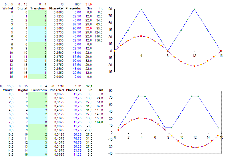
Graphical representation of the two possible declarations starting with the angle as a float value in between 0 ... X ... 16, and it's digital "code" from 0 ... 15, the focused sector of the sine wave (please have a look at the special point 4), the relative phase related to the sector origin, the absolute phase in between 360 degrees and the resulting sine waves. The added values in the right row (int) give an impression of the  integral = energy of the curve. The curves represent the 4 used points. The blue curve represents the angle from 0 ... 90 degrees.

One advantage of using Method 2 is that it allows for a slightly larger amplitude, especially in small tables, since the quarter-circles are always symmetrical with respect to the time axis when the number of points is even. Thus, for example, with 4 bits, the values are not 7, 6, 5 … -5, -6, -7—which would result in the loss of the point “-8,” even though it is possible—but rather 7.5 … -7.5, allowing all 16 points to be used while still keeping the wave symmetrical about 0. Furthermore, the single maximum value is eliminated, allowing the scale to expand further (e.g., 32.1 in the figure), which is particularly relevant at low resolutions. This effect is especially useful when the value is output directly from a converter. Potential Problems The disadvantage of Method 2—that there is no explicit zero point—is insignificant for many applications; however, it should be checked on a case-by-case basis, e.g., if a motor is to be shut off directly when phase = 0 and a true “0” is required at the converter output. It is also important to note that, in the case of post-processing the sine waves using internal digital filters, values may generally result that are larger than those specified by the interpolation points, which becomes a problem at higher amplitudes.

 To be on the safe side, one avoids amplifying the amplitude and even reduces it—for example, to minimize errors, as described above. Comparison and Conclusion: As a rule, Definition 2 is preferable. At high resolutions, the two approaches converge anyway, but the advantage of simpler vector handling remains, and there is no special treatment for the 90° case. Depending on the implementation, this would require either case differentiation or an additional bit for full modulation. The same applies to the calculation of the phase.

Analytical calculation the sine values

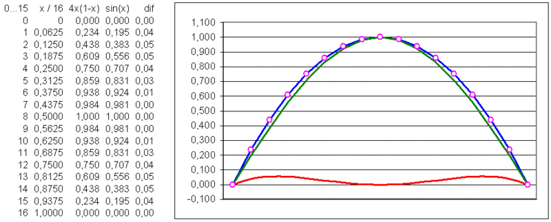
Equation : Y = x * (1 - x) / 4

Tthe sine wave can be approximated by a parabolic curve if a fast multiplication operation is available. The image shows a sine approximation and second-order approximation on the interval. The formula describes a simple approximation but is often more appropriate then a table based version. The factor 4 is chosen so that the vertex of the parabola coincides with the maximum of the sine curve. The deviation of this curve, which lies slightly above the sine curve, is no more than 12.5% and is therefore suitable for many applications where 100% accuracy is not required or where the deviation is acceptable. However the deviation can be reduced by subtracting a curve with twice the frequency.

Heuristic solution for the sine values

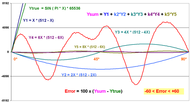
This is an optimized equation for a 16 bit sine wave with max 60 digit of error thus the sine wave has a final precision of 10 Bits. By applying correction factors derived from multiples of the excitation frequency, the harmonics in the final value can be reduced. The definition range is simply scanned by multiplying the input vector by a larger factor; starting with the 4th harmonic and higher, the resulting Y-value between two zero crossings must be manually inverted to form the respective inverse half-arc. In C, this can be done using the sign and absolute value functions; in VHDL, by utilizing the respective resulting MSBs. The resulting functions for the harmonics Y2 ... Y5 are multiplied by appropriate correction factors and added together so that the errors are minimized. Functions and errors (red, zoomed 100x) for a fifth-order approximation in the range 0...90°. In the example above, an 8-bit vector (0...255) was assumed to represent the required quarter sine wave, and 4 harmonics were used. The phase is therefore represented with 10-bit precision => 1/1024. The coefficients are: k1 = 1.0000, k2 = -0.0444, k3 = -0.0207, k4 = -0.0018, k5 = -0.00255. The deviation of the output value from the ideal sine wave (green) is approximately +/-45 digits per full-scale range (65,536 in this case), which means that, using the formula above and omitting the lower 5 bits, one can achieve a final value with an error of +/- 1 digit (~0.1% accuracy), which aligns well with the selected phase resolution

Further processsing

When the value is generated directly using formulas, the calculation can be performed at any resolution. Interpolation or filtering is not strictly necessary in these cases. However, to obtain intermediate values, the following options are available: [Edit] Interpolation The previously unused lower bits of the phase accumulator are substituted into a linear equation, where the slope and y-intercept are derived from the current and the next point. If a table is used and both the sine and the cosine are generated, the other function already specifies the slope and can be used as well. For high-speed applications, it is always worthwhile to explicitly store the slope. Using interpolation greatly reduces artifacts resulting from the limited table size.

Subsequent filtering can further improve the quality of the sine wave. A simple IIR filter, tuned to the frequency to be generated, reliably attenuates the high-frequency components—that is, the remaining “kinks” from the interpolation. The simplest implementation is a filter with binary coefficients of the form: Y(t+1) = Y(t) - Y(t)/k + sineValue/k, where k = 16, 32, 64, ...! Filtering is particularly advantageous when the frequency is switched and phase jumps need to be smoothed out.



Read about another version of Sine Wave Generation